A recent RViews article covers the use of the dplyr package to interact with SQL databases
All the code can be written in R, which dplyr then translates into SQL queries to harness the power of a database You will probably want to read the article if interested in extending the process to your own data but here is a taster from some of mine
Install and load packages
The database accessibility feature is still being developed, so currently we will need to use the development versions of dbplyr and dplyr.
# this takes  a while as needs compiling
# devtools::install_github("tidyverse/dplyr") #0.6.0
# devtools::install_github("tidyverse/dbplyr") #0.0.0.901
# devtools::install_github("rstats-db/odbc") #1.1.1.9000
# install.packages("DBI") # was 0.6-1

library(DBI)
library(odbc)
library(dplyr)
library(dbplyr)
library(plotly)
library(knitr)
Make Connection and investigate tables available
I maintain an Microsoft SQL Server which includes some tables related to the English Premier League. I have hidden the code which includes my id/password
First make the connection
con <- dbConnect(odbc::odbc(),
                   Driver    = "SQL Server Native Client 11.0",
                   Server    = "sqlb12.webcontrolcenter.com",
                   Database  = "epldb",
                   UID       = [My User ID],
                   PWD       = [My Password],
                   Port      = 1433)
Then retrieve and examine the tables. I happen to know that ‘tblPlayers’ and ‘tblPlayerClub’ are a couple of relevant ones
# There are around 500 tables but thankfully the datatables are listed first
dbListTables(con) %>% head()
## [1] "Cities" "collegeFootballRankings"
## [3] "Countries" "didCastaway"
## [5] "didTracks" "didUrl"# For these two tables the common field is PLAYERID, which will be used later
dbListFields(con, "tblPlayers")## [1] "PLAYERID" "FIRSTNAME" "LASTNAME" "PLACE" "COUNTRY"
## [6] "BIRTHDATE" "POSITION" "HEIGHT" "WEIGHT" "STICKER"
## [11] "ORDER" "PHOTO" "SoccerBase" "MatchFacts" "Who'sWho"
## [16] "ETPOS" "OPTAcode" "ETValue" "Memo" "Dead"dbListFields(con, "tblPlayerClub")## [1] "PLAYERID" "TEAMID" "JOINED"
## [4] "USJOINED" "LEFT" "FAKELEFT"
## [7] "PERMANENT" "FEE" "FEEOUT"
## [10] "MISC" "PLAYER_TEAM" "testdate"
## [13] "OldTEAMID" "SquadNo" "FirstGame"
## [16] "FirstGoal" "FirstCAution" "LastGame"
## [19] "LastGoal" "LastCaution" "SpellWithClub"
## [22] "Memo" "Out" "OutReason"
## [25] "RecordSigning" "RecordSigningClub" "RecordAgeYoungOrder"
## [28] "RecordAgeYoungYears" "RecordAgeYoungDays" "RecordAgeOldOrder"
## [31] "RecordAgeOldYears" "RecordAgeOldDays"## create some data.frames for easy manipulation, restricting to pertinent fields
players <- tbl(con, "tblPlayers") %>%
select(PLAYERID,FIRSTNAME,LASTNAME,PLACE,COUNTRY,BIRTHDATE,POSITION) %>%
as.data.frame()
playerClub <- tbl(con, "tblPlayerClub") %>%
select(PLAYERID,TEAMID,JOINED,LEFT,PERMANENT,FEE,FEEOUT,PLAYER_TEAM) %>%
as.data.frame()The ugly field names are a relic of setting up in MS Access many moons ago. Apologies
Create some example output
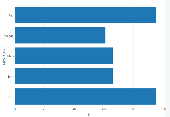
Let’s plot the most common first names of players
players %>%
  group_by(FIRSTNAME) %>%
  tally() %>%
  arrange(desc(n)) %>%
  head() %>%
  plot_ly(x=~n, y=~FIRSTNAME)
and a table of which players have appeared on the books of the most teams
players %>%
left_join(playerClub) %>% #
  group_by(PLAYERID,FIRSTNAME,LASTNAME) %>%
  tally() %>%
  filter(PLAYERID!="OWNGOAL") %>%
  ungroup() %>%
  select(name=LASTNAME,clubs=n) %>%
  arrange(desc(clubs)) %>%
  filter(clubs>6) %>%
kable()| name | clubs |
|---|---|
| Bent | 9 |
| Bellamy | 8 |
| Ben Haim | 7 |
| Cole | 7 |
| Keane | 7 |
| Nash | 7 |
| Routledge | 7 |
| Unsworth | 7 |
Ideally, this would show full name (the leader is, in fact, Marcus Bent) but attempting to combine FIRSTNAME and LASTNAME is currently causing an error
This is very much a token usage but should give some idea of the speed of interacting with a remote database and power these extra features provide