Statistics Canada make available masses of useful data from Censuses and Surveys.
One way they communicate is via twitter e.g.
library(blogdown)
shortcode("tweet", "891757886011002883")
In 2001, 31% of young adults (aged 20 to 34) were still living with their parents. Any change in 2016? Stay tuned! https://t.co/lUMBplYJWW pic.twitter.com/4CA3DvhuNw
— Statistics Canada (@StatCan_eng) July 30, 2017
Since January 2013 have also issued monthly blog posts covering a wide range of social and economic matters of interest
For each post, there is the opportunity to comment and recommend. From a cursory inspection, interaction with the public appears to have tailed off
Let’s chart this. Here are the libraries I’ll be using
library(tidyverse)
library(rvest)
library(stringr)
library(plotly)
The data needs to be scraped. I found the Chrome SelectorGadget in conjuction with rvest the best way to approach this.
There may well be a more efficient way of coding - this method relies on map and unlist - but it does the trick
At the time of writing, there have been 54 posts
N.B. If you widh to replicate the scraping you may find that they are very limiting on traffic. It took me quite a long while to obtain the data so the code is not evaluated and I reload the result from a saved file
# create functions for each variable
titleFun <- function(x) {
  # base url
  url<- paste0("http://www.statcan.gc.ca/eng/blog?widget_title=&sort_by=&sort_order=&page=",x)

  info <- read_html(url)

  title <-  info %>%
    html_nodes("#wb-main-in .mrgn-tp-sm a") %>%
    html_text()

}

recFun <- function(x) {
  url<- paste0("http://www.statcan.gc.ca/eng/blog?widget_title=&sort_by=&sort_order=&page=",x)

  info <- read_html(url)
  recs <-  info %>%
    html_nodes(".rate-statcan-recommend-btn") %>%
    html_text() %>%
    str_match_all( "[0-9]+") %>% unlist %>% as.numeric

}
commFun <- function(x) {
  url<- paste0("http://www.statcan.gc.ca/eng/blog?widget_title=&sort_by=&sort_order=&page=",x)

  info <- read_html(url)
  comments <-  info %>%
    html_nodes(".views-field-comment-count") %>%
    html_text() %>%
    str_match_all( "[0-9]+") %>% unlist  %>% as.numeric

}


dateFun <- function(x) {
  url<- paste0("http://www.statcan.gc.ca/eng/blog?widget_title=&sort_by=&sort_order=&page=",x)

  info <- read_html(url)
  comments <-  info %>%
    html_nodes(".views-field-created .field-content") %>%
    html_text()

}

# pages
pages <- 0:17


titles <- map(pages, titleFun) %>% unlist #
recommends <- map(pages, recFun) %>% unlist
comments <- map(pages, commFun) %>% unlist
dates <- map(pages, dateFun) %>% unlist

# create and save tbl
df <-tibble(titles,recommends,comments,dates)

write_csv(df, "data/canStats/blogMeta.csv")
OK Lets do a quick chart
# read in
df <- read_csv("data/canStats/blogMeta.csv")

# hack to order points correctly
df <-df %>%
  mutate(order=desc(row_number()))


 df %>%
   plot_ly(x=~order,y=~allRecommends,
           hoverinfo="text",
           text=~paste0(allDates,
                        "<br>",allTitles)) %>%
   layout(title="Statistics Canada Blog - Recommendations by Post",
          xaxis=list(title="", showticklabels = FALSE),
          yaxis=list(title="")) %>%  config(displayModeBar = F,showLink = F)
Hover for blog title
Almost two-thirds of the comments were made on the first three posts and there has been a general reduction in recommendations - though the posts remain of interest
It is not clear what the reason for this is. Obviously, the earlier posts will have been available for comment longer and regular users may not feel the need to recommend every time. There may also have been more compelling subject matter dealt with initially or just a decline in people interested in the data - though this seems unlikely over such a short time-period
One thing I have noticed, from a swift perusal, is that posts tend to be text-heavy and more an incentive to download and play with data than an exposition. I, therefore, plan to add some charts amd maps occasionally that complement both past and future StatCan posts
Here is the briefest of introductions. I’ll start with the most recent post,Mapping Canada’s wages but to keep the post short will only address one aspect of it
In June 2017, Statistics Canada released the first data on paid wages from the Job Vacancy and Wages Survey (JVWS). These data are the latest addition to the agency’s extensive labour statistics, and give significant information about the demand side of the job market: specifically, what type of workers employers have hired and how much they pay them for their labour…. Besides the scale of the survey, the fine level of detail poses a challenge. Five hundred occupations in 76 regions creates a lot of categories—and, as Ms. Do points out: “100,000 locations spread across those domains can lead to very small numbers per variable.”
Let’s break this down - although I could not immediately see all 10 broad groups
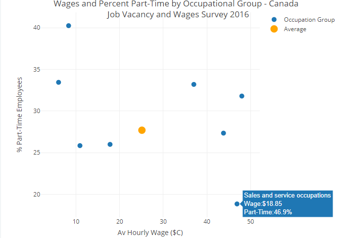
They show that nearly one-quarter of Canadian jobs in 2016 were in sales and service, a category that includes occupations such as retail salespeople, insurance agents, butchers, tour guides and janitors. Of all 10 broad occupational groups, this category also had the highest rate of part-time jobs and the lowest average wage of $18.85 per hour.
StatCan do provide some Web API’s for developers but this appears, currently, to just return the indicators available, the schedule of major economic releases and brief highlights which link to articles
The way to obtain raw data from Statcan is to make a selection of how granular you want the data and then download a csv from their CANSIM database. For this, and any subsequent, analyses on this survey I have downloaded the total file which comprises of almost 230,000 rows of 8 variables
raw <- read_csv("data/canStats/JVWS2016.csv")
glimpse(raw)
## Observations: 229,744
## Variables: 8
## $ Ref_Date                      <int> 2016, 2016, 2016, 2016, 2016, 20...
## $ GEO                           <chr> "Canada", "Canada", "Canada", "C...
## $ `Geographical classification` <chr> NA, NA, NA, NA, NA, NA, NA, NA, ...
## $ NOC4                          <chr> "Total, all occupations", "Total...
## $ STATS                         <chr> "Average full-time hourly wage p...
## $ Vector                        <chr> "v112631950", "v112631951", "v11...
## $ Coordinate                    <chr> "1.1.1", "1.1.2", "1.1.3", "1.1....
## $ Value                         <chr> "27.70", "15234260.00", "1141675...

raw %>%
  head(100) %>%
                         DT::datatable(class='compact stripe hover row-border order-column',rownames=FALSE,options= list(paging = TRUE, searching = FALSE,info=FALSE))
The format is not ideal with the STATS variable including both wage rates and employee numbers. We can get the broad groups e.g. Management occupations by restricting to ‘Coordinate’ values with 5 characters and then look at just the GEO of Canada
We then widen the data-frame so that the four different STATS groups each have their own column and we can determine the % in each broad employment group that is accounted for by part-time workers
# filter to rows required and produce a wide data.frame
wages <- raw %>%
  filter(nchar(Coordinate)==5&GEO=="Canada") %>%
  select(NOC4,STATS,Value) %>%
  spread(STATS,Value)

# simplify column names
names(wages) <- c("Group","Wage","Full","Part","Total")

# coerce most columns to numeric
cols = c(2, 3, 4, 5);
wages[,cols] = apply(wages[,cols], 2, function(x) as.numeric(x))

# calculate percent part-time
wages<- wages %>%
  mutate(Part_pc=round(100*Part/Total,1))

# create a separate overall data.frame for chart
total <- wages %>%
  filter(Group=="Total, all occupations")


# looks Ok does not show % in each occédoes nottally with groups 10
wages %>%
  plot_ly(x=~Part_pc, y=~Wage) %>%
  add_markers(name="Occupation Group", size= I(10),
              hoverinfo="text",
              text=~paste0(Group,
                           "<br>Wage:$",Wage,
                           "<br>Part-Time:",Part_pc,"%")) %>%
  add_markers(data=total,x=~Part_pc, y=~Wage, color=I("orange"),name="Average", size= I(15),
              hoverinfo="text",
              text=~paste0(Group,
                           "<br>Wage:$",Wage,
                           "<br>Part-Time:",Part_pc,"%")) %>%
  layout(title=" Wages and Percent Part-Time by Occupational Group - Canada <br> Job Vacancy and Wages Survey 2016",
         xaxis=list(title="Av Hourly Wage ($C)"),
         yaxis=list(title="% Part-Time Employees")
         ) %>%  config(displayModeBar = F,showLink = F)
Hover - for further details. The lowest wage earners - those in the pretty broad group of service occupations e.g. retail workers, janitors - are most associated with part-time work
Further work in this area could be a drill-down within each broad group and a mapped comparison by economic region. I intend to return to this in a future post