A few weeks ago I did a post on the StatCan API
I have since come across the new cancensus package, a wrapper function for CensusMapper API, in beta and not yet available on CRAN . These has been developed by the Vancouver team at MountainMath featuring Jens von Bergmann. His blog, Mountain Doodles is well worth a read - and, usefully, includes his twitter feed
You will need to get an API key to play around with the data. See the github page for instructions
Statistics Canada are in the process of rolling out information from the 2016 census, so the release of this package is particularly timely.
Please note, this is just an example of using the package with raw data and not an in depth analysis of any census information
Load up libraries and API key
# In beta so probably worth running each time
#devtools::install_github("mountainmath/cancensus")
library(cancensus) #0.1.0
library(tidyverse)
library(plotly)
library(leaflet)
library(viridis)
library(sf)


# Obtain your own key
 # options(cancensus.api_key = "Your_Census_Key")
The Basics
The workhorse at retrieving data is the get_census() function. By default, no spatial data is returned but if you want to draw maps you can return spatial data objects in either sf or sp formats. If you are planning to use this package regularly and/or are downloading lots of data you can obtain the geometry alone via get_census_geometry() and join datasets if and when required
get_census(dataset, level, regions, vectors = c(), geo_format = NA,
  labels = "detailed", use_cache = TRUE, quiet = FALSE,
  api_key = getOption("cancensus.api_key"))
There are quite a few parameters. There are some functions provided in the package to help us understand and use them
Firstly, a list of datasets available
list_census_datasets()
## # A tibble: 3 x 2
##   dataset                description
## *   <chr>                      <chr>
## 1    CA06         2006 Canada Census
## 2    CA11 2011 Canada Census and NHS
## 3    CA16         2016 Canada Census
So for the most recent data alone, we need the “CA16”" dataset
Now for the regions
#Select 2016 census
regions <- list_census_regions("CA16", quiet=TRUE)

table(regions$level)
##
##    C   CD  CMA  CSD   PR
##    1  293   49 5148   13

regions %>%
     DT::datatable(class='compact stripe hover row-border order-column',rownames=FALSE,options= list(paging = TRUE, searching = TRUE,info=FALSE))
There are 5 levels of geography which can be called: country, province, census metropolitan area, census and census sub-district. Please note, that the data grouping within that can be finer - as we will see later
The table makes it easy to select a region of interest. Just use the search facility
Similarly we can set the full set of vectors (tables)
list_census_vectors("CA16", quiet=TRUE) %>%
     DT::datatable(class='compact stripe hover row-border order-column',rownames=FALSE,options= list(paging = TRUE, searching = TRUE,info=FALSE))
It can be better to use a search function which, if unable to find a given search term, will suggest the correct spelling to use when possible
Income Data
Income data forms the most recent census data release, so let’s see what there is available to investigate
search_census_vectors('Income', 'CA16') %>%
     DT::datatable(class='compact stripe hover row-border order-column',rownames=FALSE,options= list(paging = TRUE, searching = TRUE,info=FALSE))
##
Downloading: 3.6 kB
Downloading: 3.6 kB
Downloading: 7.6 kB
Downloading: 7.6 kB
Downloading: 12 kB
Downloading: 12 kB
Downloading: 12 kB
Downloading: 12 kB
Downloading: 16 kB
Downloading: 16 kB
Downloading: 20 kB
Downloading: 20 kB
Downloading: 20 kB
Downloading: 20 kB
Downloading: 24 kB
Downloading: 24 kB
Downloading: 28 kB
Downloading: 28 kB
Downloading: 32 kB
Downloading: 32 kB
Downloading: 32 kB
Downloading: 32 kB
Downloading: 32 kB
Downloading: 32 kB
Downloading: 37 kB
Downloading: 37 kB
Downloading: 37 kB
Downloading: 37 kB
Pretty much at random, let’s look at “Median total income of economic families in 2015 ($), v_CA16_2447”“, which is on page 9 of the above table
I will choose the Greater Toronto Area (35535), where I lived up until a few years ago: initially using a broad brush by obtaining the census sub-districts and downloading the spatial data in the sf format
df <- get_census(dataset='CA16', regions=list(CMA="35535"), vectors=c("v_CA16_2447"), level='CSD', geo_format = "sf")

glimpse(df)
## Observations: 24
## Variables: 15
## $ `Shape Area`                                                        <dbl> ...
## $ Type                                                                <fctr> ...
## $ Dwellings                                                           <int> ...
## $ Households                                                          <int> ...
## $ GeoUID                                                              <chr> ...
## $ Population                                                          <int> ...
## $ name                                                                <chr> ...
## $ `Adjusted Population (previous Census)`                             <int> ...
## $ PR_UID                                                              <chr> ...
## $ CSD_UID                                                             <chr> ...
## $ CMA_UID                                                             <chr> ...
## $ `Region Name`                                                       <fctr> ...
## $ `Area (sq km)`                                                      <dbl> ...
## $ `v_CA16_2447: Median total income of economic families in 2015 ($)` <dbl> ...
## $ geometry                                                            <simple_feature> ...

colnames(df)[14] <- "Income"
If the data has been downloaded previously it is cached locally - a particular benefit with large datsets - this one has only 21 rows
The penultimate column is a bit of a mouthful which I have amended to be called “Income”
Lets look at mapping this field in leaflet. I like to look at variation first to help determine how to bin
df %>%
plot_ly(x=~Income)
One outlier. Does this make sense?
df %>%
  arrange(Income) %>%
  select(-geometry) %>%
  select(Population,name,Income)  %>%
     DT::datatable(class='compact stripe hover row-border order-column',rownames=FALSE,options= list(paging = TRUE, searching = TRUE,info=FALSE))
NB not sure why the geometry field still shows up
A small population of First Nations People clarifies the position. Four groupings appears appropriate
Now lets do an exploratory map in leaflet. This requires transforming the co-ordinates in df$geometry to a different projection. Just one line of code!
# Select colours for the four bins
pal <- colorBin(palette = viridisLite::inferno(4),
                    domain = df$Income,
                bins=c(0,100000,110000,120000,150000))


# minimal map
df %>%
  st_transform(crs = "+init=epsg:4326") %>% # from sf package
  leaflet() %>%
  addProviderTiles(provider = "CartoDB.Positron") %>%
   addPolygons(
     label= ~name,

               color = ~ pal(Income)
   ) %>%
    addLegend("bottomleft",
              pal = pal,
              values = ~ Income,
              title = "Median total income of <br> economic families in 2015",
              opacity = 0.5)
Hover over an area to see it’s name
I would probably use a different colour scheme for a more polished output and add highlight parameters
Not entirely what I would have expected - although the total spread is not all that great and the tendency of the west sides of cities to be populated by the more affluent is confirmed. Probably worth looking at the definition of the underlying table more closely.
OK let’s look in more detail at the City of Toronto, which accounts for roughly half the population of the GTA. This time I will go down to census tract (CT) level for much finer detail
toronto <-  get_census(dataset='CA16', regions=list(CMA="3520"), vectors=c("v_CA16_2447"), level='CT', geo_format = "sf")
colnames(toronto)[14] <- "Income"
toronto %>%
plot_ly(x=~Income)
Now have 572 areas, with only a couple having a population of over 12,000
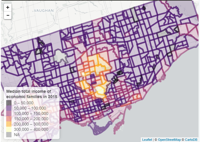
I’d quite like to highlight the extreme wealth areas so have upped the bands to number six
pal <- colorBin(palette = viridisLite::inferno(6),
                    domain = df$Income,
                bins=c(0,50000,100000,150000,200000,300000,400000))


toronto %>%
  st_transform(crs = "+init=epsg:4326") %>%
  leaflet() %>%
  addProviderTiles(provider = "CartoDB.Positron") %>%
   addPolygons(
     label= ~ paste0("$",Income),

               color = ~ pal(Income)
   ) %>%
    addLegend("bottomleft",
              pal = pal,
              values = ~ Income,
              title = "Median total income of <br> economic families in 2015",
              opacity = 0.5)
Zoom and pan as desired. The tracts are just ids, so The hover shows the mean income value instead
This shows that mapping does appear to tell a story. The bulk of the tracts are under $100,000 income; the lakeside tends to be a bit higher on the income scale; and the most affluent areas are in mid-town, with another up-market area in the West. The Rosedale district is home to some lovely abodes but is not far, physically from one of the poorest areas in the city, St. James Town
Let’s obtain the equivalent agglomeration for the Greater Vancouver region
vancouver <-  get_census(dataset='CA16', regions=list(CMA="5915"), vectors=c("v_CA16_2447"), level='CT', geo_format = "sf")
colnames(vancouver)[14] <- "Income"
vancouver %>%
plot_ly(x=~Income)
pal <- colorBin(palette = viridisLite::inferno(5),
domain = df$Income,
bins=c(0,60000,80000,100000,120000,200000))
# minimal map
vancouver %>%
st_transform(crs = "+init=epsg:4326") %>%
leaflet() %>%
addProviderTiles(provider = "CartoDB.Positron") %>%
addPolygons(
label= ~ paste0("$",Income),
opacity = 0.7,
color = ~ pal(Income)
) %>%
addLegend("bottomleft",
pal = pal,
values = ~ Income,
title = "Median total income of <br> economic families in 2015",
opacity = 0.5) Definitely, a different look to Toronto . West Vancouver (the NW sector of this map) is a notoriously rich area - but a lot of that is wealth rather than income. House values are high but there are quite a lot of retired people there. This would make a good follow-up exercise
The income distribution - at least at this geographic level - is surprisingly Gaussian. Maybe less bankers than in Toronto!?
So a first, quick pass at a great package. Any serious analysis of the implications of the census results would need to clarify definitions and take other factors into account. Luckily there are many more tables available to do just that